Tutorial
Here we present an example genotype-phenotype (G/P) analysis with GPSEA. We assume GPSEA was installed as described in the Setup section and we encourage the users to execute the tutorial code in a Jupyter notebook or a similar interactive environment.
Background
In this tutorial, we analyze a cohort of individuals with pathogenic variants in TBX5 leading to Holt-Oram syndrome MIM:142900.
Holt-Oram syndrome is an autosomal dominant disorder characterized by upper limb defects, congenital heart defects, and arrhythmias (PMID:38336121). It has been observed in the literature that congenital defects of the ventricular and atrial septum are more common in the truncating than in the missense variants (PMID:30552424). Additionally, upper limb defects are more frequent in patients with protein-truncating variants (PMID:38336121).
We curated the literature and created a GA4GH phenopacket for each affected individual. The phenopackets are published in Phenopacket Store.
Analysis
A typical GPSEA analysis will consist of several steps. Starting with a collection of phenopackets, we perform input Q/C and functional variant annotation to prepare a cohort. With the cohort on hand, we generate reports with summary statistics, variant distributions, and most common Human Phenotype Ontology (HPO) terms or measurements. We then configure the methods for partitioning the cohort into genotype and phenotype classes, to test for possible associations between the classes. We finalize the analysis by statistical testing and evaluation of the results.
Inputs and Q/C
Gene and transcript
For the analysis, the MANE transcript (i.e., the “main” biomedically relevant transcript of a gene) should be chosen unless there is a specific reason not to (which should occur rarely if at all).
In the case of TBX5 the MANE transcript is NM_181486.4. Note that the trascript identifier (NM_181486) and the version (4) are both required. A good way to find the MANE transcript is to search on the gene symbol (e.g., TBX5) in ClinVar and to choose a variant that is specifically located in the gene. The MANE transcript will be displayed here (e.g., NM_181486.4(TBX5):c.1221C>G (p.Tyr407Ter)).
We additionally need the corresponding protein identifier. A good way to find this is to search on the transcript id in NCBI Nucleotide. In our case, search on NM_181486.4 will bring us to this page. If we search within this page for “NP_”, this will bring us to the corresponding protein accession NP_852259.1.
>>> cohort_name = 'TBX5'
>>> tx_id = 'NM_181486.4'
>>> px_id = 'NP_852259.1'
Human Phenotype Ontology
The analysis in this tutorial needs to access Human Phenotype Ontology (HPO). We use HPO toolkit to load the version v2024-07-01 of HPO:
>>> import hpotk
>>> store = hpotk.configure_ontology_store()
>>> hpo = store.load_minimal_hpo(release='v2024-07-01')
Tip
Use the latest HPO release by omitting the release option from the loader method.
Load phenopackets
Now we will load the samples to analyze. We will use the cohort of 156 individuals with mutations in TBX5 whose clinical signs and symptoms were encoded into HPO terms and stored in Phenopacket Store.
>>> from ppktstore.registry import configure_phenopacket_registry
>>> phenopacket_registry = configure_phenopacket_registry()
>>> with phenopacket_registry.open_phenopacket_store("0.1.20") as ps:
...     phenopackets = tuple(ps.iter_cohort_phenopackets(cohort_name))
>>> len(phenopackets)
156
We loaded 156 phenopackets which need further preprocessing to prepare for the analysis.
We will compute functional annotations for the mutations and then include the individuals into
a Cohort:
>>> from gpsea.preprocessing import configure_caching_cohort_creator, load_phenopackets
>>> cohort_creator = configure_caching_cohort_creator(hpo)
>>> cohort, validation = load_phenopackets(
...     phenopackets=phenopackets,
...     cohort_creator=cohort_creator,
... )
Individuals Processed: ...
and we will check that there are no Q/C issues:
>>> validation.summarize()
Validated under none policy
No errors or warnings were found
We loaded the patient data into a cohort which is ready for the next steps.
See also
Here we show how to create a Cohort from phenopackets.
See Input data section to learn how to create a cohort from another inputs.
Explore cohort
Once the genotype and phenotype has been standardized, we can generate reports to gain insight for the cohort data.
Show cohort summary
The cohort summary report provides an overview about the most common HPO terms, variants, diseases, and variant effects:
>>> from gpsea.view import CohortViewer
>>> viewer = CohortViewer(hpo)
>>> report = viewer.process(cohort=cohort, transcript_id=tx_id)
>>> report
GPSEA cohort analysis
Successfully loaded 156 individuals. 46 were recorded as male, 56 as female, and 54 as unknown sex. No information about individuals' vital status was reported. 52 individuals had disease onset information and 0 had information about the age of last encounter.
No errors encountered.
HPO terms
| n | HPO Term |
|---|---|
| 50 | Atrial septal defect |
| 41 | Ventricular septal defect |
| 40 | Hypoplasia of the radius |
| 36 | Triphalangeal thumb |
| 32 | Short thumb |
| 32 | Absent thumb |
| 30 | Abnormal carpal morphology |
| 27 | Secundum atrial septal defect |
| 15 | Absent radius |
| 14 | Cardiac conduction abnormality |
Measurements
No data regarding measurement assays were provided.Diseases
The cohort members were diagnosed with 1 disease.| n | Disease |
|---|---|
| 156 | Holt-Oram syndrome |
Variants
A total of 53 unique variants were identified in the cohort. Variants were annotated with respect to NM_181486.4.
| n | Variant key | HGVS | Variant Class |
|---|---|---|---|
| 22 | 12_114385521_114385521_C_T | c.710G>A (p.Arg237Gln) | MISSENSE_VARIANT |
| 20 | 12_114401830_114401830_C_T | c.238G>A (p.Gly80Arg) | MISSENSE_VARIANT |
| 8 | 12_114385563_114385563_G_A | c.668C>T (p.Thr223Met) | MISSENSE_VARIANT |
| 6 | 12_114398675_114398675_G_T | c.408C>A (p.Tyr136Ter) | STOP_GAINED |
| 5 | 12_114399514_114399514_A_C | c.361T>G (p.Trp121Gly) | MISSENSE_VARIANT, SPLICE_REGION_VARIANT |
| 5 | 12_114398682_114398682_C_CG | c.400dup (p.Arg134ProfsTer49) | FRAMESHIFT_VARIANT |
| 5 | 12_114403792_114403792_C_CG | c.106_107insC (p.Ser36ThrfsTer25) | FRAMESHIFT_VARIANT |
| 4 | 12_114385474_114385474_A_G | c.755+2T>C (None) | SPLICE_DONOR_VARIANT |
| 4 | 12_114398656_114398656_C_CG | c.426dup (p.Ala143ArgfsTer40) | FRAMESHIFT_VARIANT |
| 4 | 12_114403798_114403798_G_GC | c.100dup (p.Ala34GlyfsTer27) | FRAMESHIFT_VARIANT |
Variant effects
The effects were predicted for NM_181486.4
| Variant effect | Count |
|---|---|
| MISSENSE_VARIANT | 85 (50%) |
| FRAMESHIFT_VARIANT | 38 (22%) |
| STOP_GAINED | 19 (11%) |
| SPLICE_REGION_VARIANT | 10 (6%) |
| SPLICE_DONOR_VARIANT | 7 (4%) |
| INFRAME_INSERTION | 2 (1%) |
| STOP_RETAINED_VARIANT | 2 (1%) |
| SPLICE_ACCEPTOR_VARIANT | 2 (1%) |
| SPLICE_DONOR_5TH_BASE_VARIANT | 2 (1%) |
| INTRON_VARIANT | 2 (1%) |
| INFRAME_DELETION | 1 (1%) |
Plot distribution of variants with respect to the protein sequence
We can use CohortArtist to plot the distribution of variants
with respect to the encoded protein on
a Matplotlib Axes:
>>> import matplotlib.pyplot as plt
>>> from gpsea.view import configure_default_cohort_artist
>>> cohort_artist = configure_default_cohort_artist()
>>> fig, ax = plt.subplots(figsize=(15, 8))
>>> cohort_artist.draw_protein(
...     cohort=cohort,
...     protein_id=px_id,
...     ax=ax,
... )
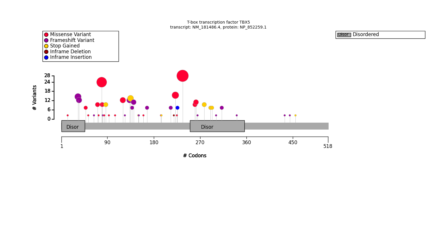
The diagram plots the location of the variants with respect to the protein sequence. The variant location is represented by a “lollipop”. The lollipop color represents the predicted variant effect and the lollipop size corresponds to the allele count within the cohort. The diagram also highlights the protein features (domains, repeats, etc.).
Summarize all variant alleles
We can prepare a table of all variant alleles that occur in the cohort.
Each table row corresponds to a single allele and lists the variant key, the predicted effect on the transcript (cDNA) and protein of interest, the variant effects, and the number of patients who present with one or more variant alleles (Count):
>>> from gpsea.view import CohortVariantViewer
>>> viewer = CohortVariantViewer(tx_id=tx_id)
>>> report = viewer.process(cohort=cohort)
>>> report
Variant alleles
| Count | Variant key | HGVS | Overlapping Exons | Effects |
|---|---|---|---|---|
| 22 | 12_114385521_114385521_C_T | c.710G>A (p.Arg237Gln) | 7 | missense |
| 20 | 12_114401830_114401830_C_T | c.238G>A (p.Gly80Arg) | 3 | missense |
| 8 | 12_114385563_114385563_G_A | c.668C>T (p.Thr223Met) | 7 | missense |
| 6 | 12_114398675_114398675_G_T | c.408C>A (p.Tyr136Ter) | 5 | stop gained |
| 5 | 12_114399514_114399514_A_C | c.361T>G (p.Trp121Gly) | 4 | missense, splice region |
| 5 | 12_114403792_114403792_C_CG | c.106_107insC (p.Ser36ThrfsTer25) | 2 | frameshift |
| 5 | 12_114398682_114398682_C_CG | c.400dup (p.Arg134ProfsTer49) | 5 | frameshift |
| 4 | 12_114403798_114403798_G_GC | c.100dup (p.Ala34GlyfsTer27) | 2 | frameshift |
| 4 | 12_114385522_114385522_G_A | c.709C>T (p.Arg237Trp) | 7 | missense |
| 4 | 12_114366360_114366360_C_T | c.787G>A (p.Val263Met) | 8 | missense |
| 4 | 12_114385474_114385474_A_G | c.755+2T>C (-) | - | splice donor |
| 4 | 12_114398656_114398656_C_CG | c.426dup (p.Ala143ArgfsTer40) | 5 | frameshift |
| 3 | 12_114403798_114403799_GC_G | c.100del (p.Ala34ProfsTer32) | 2 | frameshift |
| 3 | 12_114399613_114399613_T_A | c.262A>T (p.Lys88Ter) | 4 | stop gained |
| 3 | 12_114401827_114401827_T_A | c.241A>T (p.Arg81Trp) | 3 | missense, splice region |
| 3 | 12_114401853_114401853_G_T | c.215C>A (p.Thr72Lys) | 3 | missense |
| 3 | 12_114366312_114366312_G_A | c.835C>T (p.Arg279Ter) | 8 | stop gained |
| 3 | 12_114366366_114366366_T_A | c.781A>T (p.Ser261Cys) | 8 | missense |
| 3 | 12_114385475_114385475_C_T | c.755+1G>A (-) | - | splice donor |
| 2 | 12_114366207_114366208_GC_G | c.939del (p.Gln315ArgfsTer79) | 8 | frameshift |
| 2 | 12_114403754_114403754_G_T | c.145C>A (p.Gln49Lys) | 2 | missense, splice region |
| 2 | 12_114385521_114385521_C_G | c.710G>C (p.Arg237Pro) | 7 | missense |
| 2 | 12_114398666_114398667_TG_T | c.416del (p.Pro139GlnfsTer11) | 5 | frameshift |
| 2 | 12_114385550_114385550_A_AATTATTCTCAG | c.680_681insCTGAGAATAAT (p.Ile227_Glu228insTer) | 7 | inframe insertion, stop retainined |
| 2 | 12_114366274_114366274_G_T | c.873C>A (p.Tyr291Ter) | 8 | stop gained |
| 2 | 12_114366267_114366267_C_A | c.880G>T (p.Glu294Ter) | 8 | stop gained |
| 2 | 12_114394762_114394763_CA_C | c.641del (p.Val214GlyfsTer12) | 6 | frameshift |
| 2 | 12_114398578_114398579_CA_C | c.504del (p.Phe168LeufsTer6) | 5 | frameshift |
| 2 | 12_114398568_114398568_C_A | c.510+5G>T (-) | - | splice donor 5th base, intronic |
| 1 | 12_114399594_114399594_A_C | c.281T>G (p.Leu94Arg) | 4 | missense |
| 1 | 12_114366348_114366349_CT_C | c.798del (p.Val267TrpfsTer127) | 8 | frameshift |
| 1 | 12_114403859_114403859_G_T | c.40C>A (p.Pro14Thr) | 2 | missense |
| 1 | 12_114399625_114399629_ACATC_A | c.246_249del (p.Met83PhefsTer6) | 4 | frameshift |
| 1 | 12_114401907_114401907_A_G | c.161T>C (p.Ile54Thr) | 3 | missense |
| 1 | 12_114394820_114394820_C_G | c.584G>C (p.Gly195Ala) | 6 | missense |
| 1 | 12_114385553_114385553_C_A | c.678G>T (p.Lys226Asn) | 7 | missense |
| 1 | 12_114398632_114398632_G_A | c.451C>T (p.Gln151Ter) | 5 | stop gained |
| 1 | 12_114398708_114398709_GC_G | c.374del (p.Gly125AlafsTer25) | 5 | frameshift |
| 1 | 12_114356064_114356065_TA_T | c.1024del (p.Tyr342ThrfsTer52) | 9 | frameshift |
| 1 | 12_114401921_114401921_C_G | c.148-1G>C (-) | - | splice acceptor |
| 1 | 12_114398602_114398602_T_G | c.481A>C (p.Thr161Pro) | 5 | missense |
| 1 | 12_114355755_114355756_TG_T | c.1333del (p.His445MetfsTer137) | 9 | frameshift |
| 1 | 12_114401873_114401874_TA_T | c.194del (p.Leu65GlnfsTer10) | 3 | frameshift |
| 1 | 12_114398626_114398627_CG_C | c.456del (p.Val153SerfsTer21) | 5 | frameshift |
| 1 | 12_114399633_114399633_C_G | c.243-1G>C (-) | - | splice acceptor |
| 1 | 12_114399559_114399559_T_C | c.316A>G (p.Ile106Val) | 4 | missense |
| 1 | 12_114401846_114401846_C_G | c.222G>C (p.Met74Ile) | 3 | missense |
| 1 | 12_114366241_114366242_CT_C | c.905del (p.Gln302ArgfsTer92) | 8 | frameshift |
| 1 | 12_114355723_114355723_G_A | c.1366C>T (p.Gln456Ter) | 9 | stop gained |
| 1 | 12_114355784_114355785_CA_C | c.1304del (p.Leu435ArgfsTer147) | 9 | frameshift |
| 1 | 12_114394817_114394817_G_C | c.587C>G (p.Ser196Ter) | 6 | stop gained |
| 1 | 12_114399622_114399622_G_T | c.253C>A (p.Pro85Thr) | 4 | missense |
| 1 | 12_114394743_114394746_TGTG_T | c.658_660del (p.His220del) | 6 | inframe deletion |
Partition the cohort by genotype and phenotype
Testing for a genotype-phenotype association uses genotype and phenotype as variables.
In GPSEA, the variable value for an individual is computed
either by a Classifier
or by a PhenotypeScorer.
A Classifier assigns the individual into a class,
whereas a PhenotypeScorer computes a continuous score.
The classifiers and scorers are applied on all individuals of the cohort
and the resulting variable distributions are then assessed by a statistical test.
In GPSEA, genotype is always treated as a class and a genotype Classifier is a prerequisite for each analysis. However, there is much more flexibility on the phenotype part, where either a Classifier or a PhenotypeScorer can be used to compute the values, depending on the analysis goals.
In this tutorial section, we first configure a Classifier for assigning the individuals into a genotype class, and we follow with generating classifiers for testing the presence or exclusion of HPO terms in the individuals.
Partition by genotype
In context of the tutorial, we assign each cohort member into a class depending on presence of a single allele of a missense or truncating variant (e.g. frameshift, stop gain, or splice site region):
>>> from gpsea.model import VariantEffect
>>> from gpsea.analysis.predicate import variant_effect, anyof
>>> from gpsea.analysis.clf import monoallelic_classifier
>>> is_missense = variant_effect(VariantEffect.MISSENSE_VARIANT, tx_id)
>>> truncating_effects = (
...    VariantEffect.TRANSCRIPT_ABLATION,
...    VariantEffect.TRANSCRIPT_TRANSLOCATION,
...    VariantEffect.FRAMESHIFT_VARIANT,
...    VariantEffect.START_LOST,
...    VariantEffect.STOP_GAINED,
...    VariantEffect.SPLICE_DONOR_VARIANT,
...    VariantEffect.SPLICE_ACCEPTOR_VARIANT,
...    # more effects could be listed here ...
... )
>>> is_truncating = anyof(variant_effect(e, tx_id) for e in truncating_effects)
>>> gt_clf = monoallelic_classifier(
...     a_predicate=is_missense,
...     b_predicate=is_truncating,
...     a_label="Missense", b_label="Truncating",
... )
>>> gt_clf.class_labels
('Missense', 'Truncating')
This is a lot of code, and detailed explanations and examples are available in the Partitioning section. For now, it is enough to know that the gt_clf will assign the individuals into Missense or Truncating class. The individuals with the number of missense (or truncating) variants different than one will be omitted from the analysis.
Partition by phenotype
We use HPO terms to assign the individuals into phenotype classes, according to the term’s presence or exclusion. The testing leverages the True path rule of ontologies.
We now prepare the classifiers for assigning into phenotype classes:
>>> from gpsea.analysis.clf import prepare_classifiers_for_terms_of_interest
>>> pheno_clfs = prepare_classifiers_for_terms_of_interest(
...     cohort=cohort,
...     hpo=hpo,
... )
Multiple testing correction
By default, GPSEA performs a test for each HPO term used to annotate at least one individual in the cohort, and there are 369 such terms in TBX5 cohort:
>>> len(pheno_clfs)
369
However, testing multiple hypothesis on the same dataset increases the chance of receiving false positive result. Luckily, GPSEA simplifies the application of an appropriate multiple testing correction.
For general use, we recommend using a combination
of a phenotype MT filter (PhenotypeMtcFilter) with a multiple testing correction.
Phenotype MT filter chooses the HPO terms to test according to several heuristics, which
reduce the multiple testing burden and focus the analysis
on the most interesting terms (see HPO MT filter for more info).
Then the multiple testing correction, such as Bonferroni or Benjamini-Hochberg,
is used to control the family-wise error rate or the false discovery rate.
See Multiple-testing correction for more information.
>>> from gpsea.analysis.pcats import configure_hpo_term_analysis
>>> analysis = configure_hpo_term_analysis(hpo)
configure_hpo_term_analysis() configures the analysis
that uses HPO MTC filter (HpoMtcFilter) for selecting HPO terms of interest,
Fisher Exact test for computing nominal p values, and Benjamini-Hochberg for multiple testing correction.
Statistical testing
Now we can perform the testing and evaluate the results.
>>> result = analysis.compare_genotype_vs_phenotypes(
...     cohort=cohort,
...     gt_clf=gt_clf,
...     pheno_clfs=pheno_clfs,
... )
>>> result.total_tests
17
We only tested 17 HPO terms. This is despite the individuals being collectively annotated with 369 direct and indirect HPO terms
>>> len(result.phenotypes)
369
We can show the reasoning behind not testing 352 (369 - 17) HPO terms by exploring the phenotype MTC filtering report:
>>> from gpsea.view import MtcStatsViewer
>>> mtc_viewer = MtcStatsViewer()
>>> mtc_report = mtc_viewer.process(result)
>>> mtc_report
Phenotype testing report
- Phenotype MTC filter: HPO MTC filter
- Multiple testing correction: fdr_bh
| Code | Reason | Count |
|---|---|---|
| HMF01 | Skipping term with maximum frequency that was less than threshold 0.4 | 19 |
| HMF08 | Skipping general term | 48 |
| HMF09 | Skipping term with maximum annotation frequency that was less than threshold 0.4 | 285 |
and these are the tested HPO terms ordered by the p value corrected with the Benjamini-Hochberg procedure:
>>> from gpsea.view import summarize_hpo_analysis
>>> summary_df = summarize_hpo_analysis(hpo, result)
>>> summary_df
Missense |
Truncating |
Corrected p values |
p values |
|
|---|---|---|---|---|
Ventricular septal defect [HP:0001629] |
31/60 (52%) |
29/29 (100%) |
9.550859422122477e-06 |
5.618152601248516e-07 |
Hypoplasia of the radius [HP:0002984] |
30/62 (48%) |
10/27 (37%) |
1.0 |
0.3614379675325876 |
Atrial septal defect [HP:0001631] |
42/44 (95%) |
38/38 (100%) |
1.0 |
0.49653718759409815 |
Secundum atrial septal defect [HP:0001684] |
14/35 (40%) |
13/40 (32%) |
1.0 |
0.6304400561799244 |
Abnormal thumb morphology [HP:0001172] |
30/30 (100%) |
56/56 (100%) |
1.0 |
1.0 |
Abnormal finger morphology [HP:0001167] |
36/36 (100%) |
56/56 (100%) |
1.0 |
1.0 |
Abnormal digit morphology [HP:0011297] |
38/38 (100%) |
59/59 (100%) |
1.0 |
1.0 |
Abnormal atrial septum morphology [HP:0011994] |
43/43 (100%) |
38/38 (100%) |
1.0 |
1.0 |
Abnormal cardiac atrium morphology [HP:0005120] |
43/43 (100%) |
38/38 (100%) |
1.0 |
1.0 |
Abnormal long bone morphology [HP:0011314] |
44/44 (100%) |
19/19 (100%) |
1.0 |
1.0 |
Abnormal hand morphology [HP:0005922] |
53/53 (100%) |
41/41 (100%) |
1.0 |
1.0 |
Aplasia/hypoplasia of the extremities [HP:0009815] |
55/55 (100%) |
44/44 (100%) |
1.0 |
1.0 |
Aplasia/hypoplasia involving bones of the upper limbs [HP:0006496] |
55/55 (100%) |
44/44 (100%) |
1.0 |
1.0 |
Aplasia/hypoplasia involving bones of the extremities [HP:0045060] |
55/55 (100%) |
44/44 (100%) |
1.0 |
1.0 |
Aplasia/hypoplasia involving the skeleton [HP:0009115] |
56/56 (100%) |
45/45 (100%) |
1.0 |
1.0 |
Abnormal cardiac septum morphology [HP:0001671] |
62/62 (100%) |
50/50 (100%) |
1.0 |
1.0 |
Abnormal appendicular skeleton morphology [HP:0011844] |
64/64 (100%) |
60/60 (100%) |
1.0 |
1.0 |
We see that several HPO terms are significantly associated with presence of a truncating variant in TBX5. For example, Ventricular septal defect was observed in 31/60 (52%) patients with a missense variant but it was observed in 29/29 (100%) patients with a truncating variant. Fisher exact test computed a p value of 5.61e-7 and the p value corrected by Benjamini-Hochberg procedure is 9.55e-6.
Conclusion
We showed the high-level structure of genotype-phenotype association analysis using GPSEA and we found an association between truncating TBX5 variants and Ventricular septal defect.
This is just one of many analysis types that are possible with GPSEA. Please refer to the User guide (next section) to learn more.