Visualizing Knowledge Graphs

Shawn T O’Neil

Vignette updated: Aug-19-2025

monarchr supports a large number of plotting frameworks compatible with tidygraph and igraph, including ggraph, visNetwork, and threejs. Included are a basic plot() for knowledge graphs via ggraph, and a cytoscape() function to export a graph to a running Cytoscape instance via RCy3.

As usual, we begin by loading the monarchr package, along with tidygraph and dplyr which tend to be useful.

library(monarchr)
library(tidygraph)
library(dplyr)

Basic plot()

The basic plot() function is a wrapper around ggraph. By default, node color tracks pcategory and edge color predicate, though these can be changed with the node_color and edge_color properties.

While node_shape and edge_linetype can also be changed, they default to namespace (commonly indicating the node’s data source) and primary_knowledge_source (commonly indicating the edge’s data source). Here we see that these nodes are part of MONDO and HGNC, and the relationships between them are sourced from MONDO as well as OMIM and Orphanet.

data(eds_marfan_kg)

g <- eds_marfan_kg |>
  fetch_nodes(query_ids = c("MONDO:0017310")) |>
  expand(predicates = "biolink:subclass_of", direction = "in", transitive = TRUE) |>
  expand(categories = "biolink:Gene")

plot(g)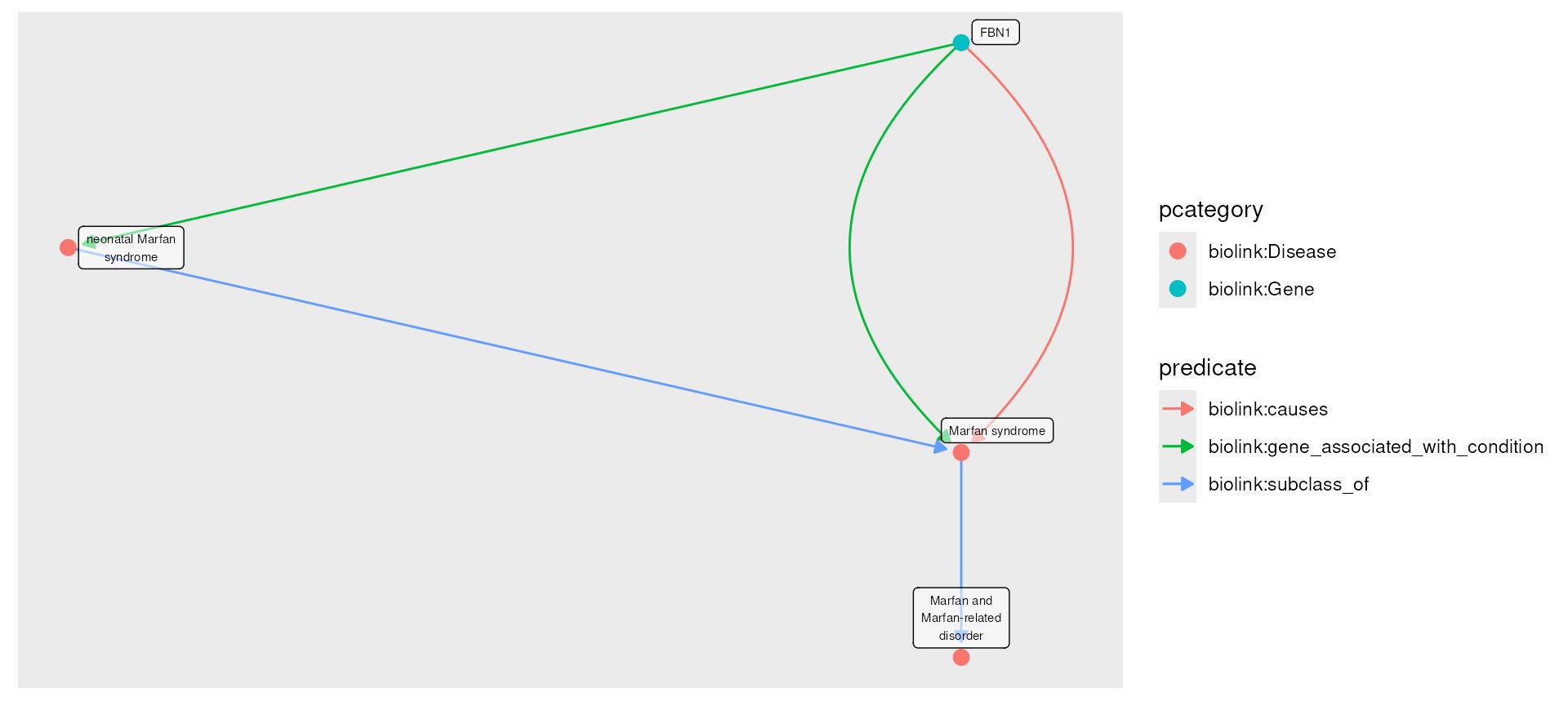

In this example we first fetch Neonatal Marfan Syndrome, Brittle Cornea Syndrome, and their direct phenotypes. We then take the join of these two graphs, compute the degree of each node and filter to only those nodes with degree > 2, indicating only phenotypes connected with both. For plotting, we use edge_color set to frequency_qualifier, but we recode those by their interpretation. The edge_color and node_color parameters simply pass their unquoted arguments to geom_node_point and geom_edge_fan ggraph layers.

mar_phenos <- eds_marfan_kg |> 
  fetch_nodes(query_ids = c("MONDO:0017309")) |>
  expand(categories = "biolink:PhenotypicFeature") 

bcs_phenos <- eds_marfan_kg |> 
  fetch_nodes(query_ids = c("MONDO:0009242")) |>
  expand(categories = "biolink:PhenotypicFeature")

both <- kg_join(mar_phenos, bcs_phenos) 

shared <- both |>
  activate(nodes) |>
  mutate(degree = igraph::degree(both)) |>
  filter(degree > 1) |>
  activate(edges) |>
  mutate(frequency_qualifier = factor(frequency_qualifier, 
                                      levels = c("HP:0040281", "HP:0040282", "HP:0040283"),
                                      labels = c("very_frequent", "frequent", "occasional")))

plot(shared, edge_color = frequency_qualifier)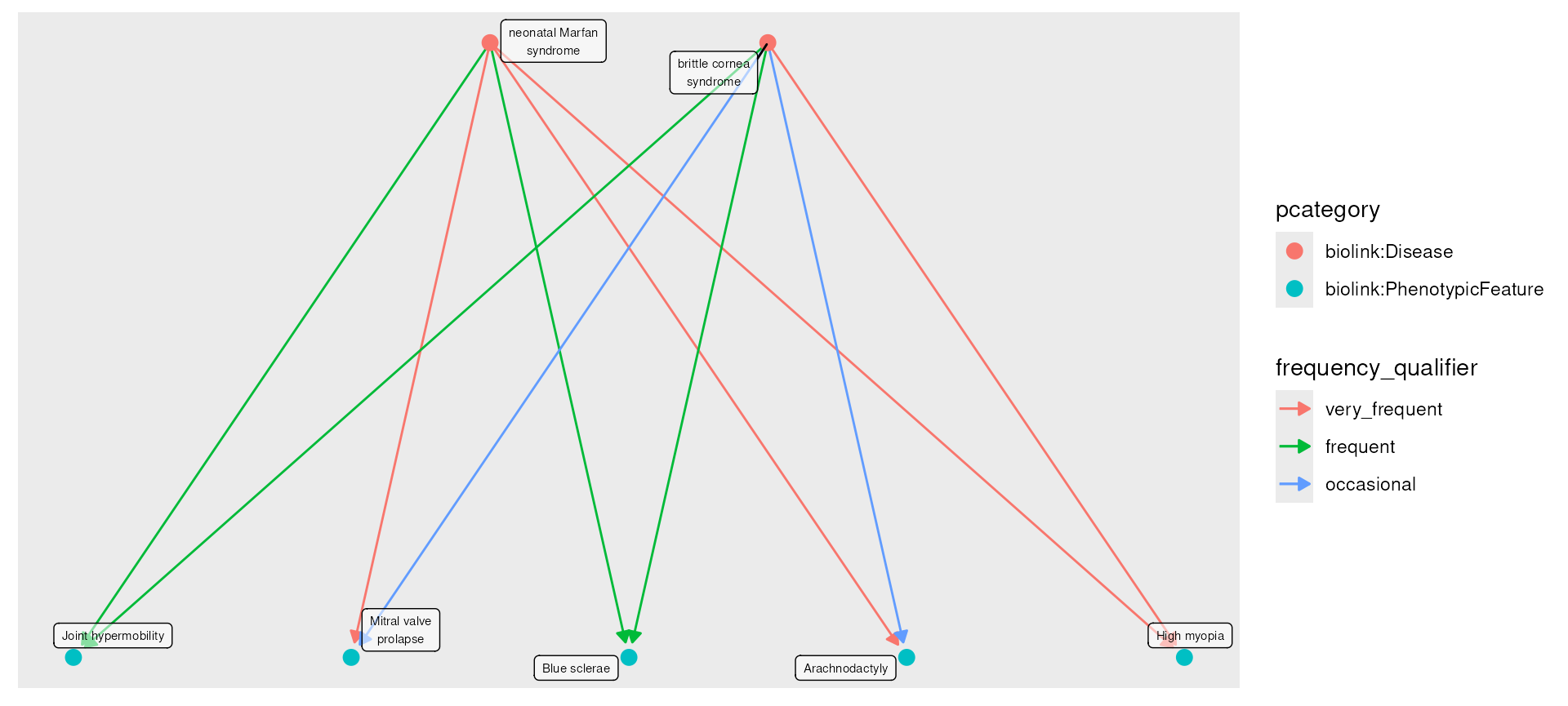

Tidygraph utilities support easy modification of node and edge tables, breadth- and depth-first maps, and other graph-centric methods, all of which may be visualized in creative ways.

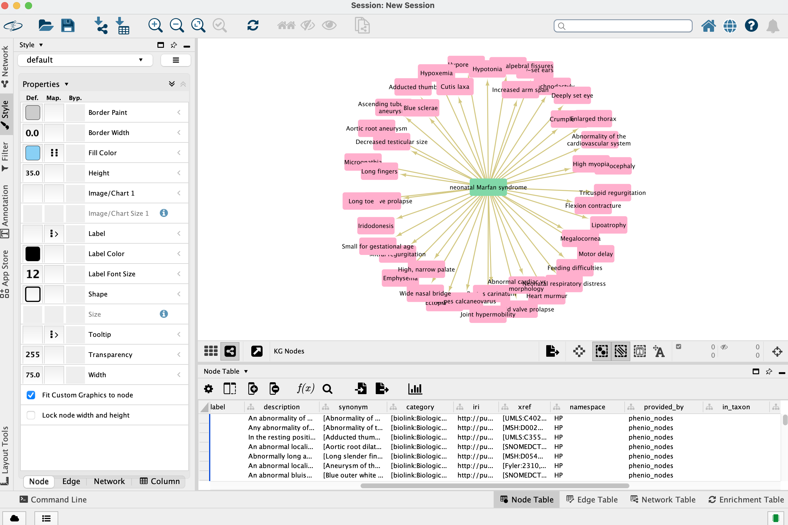
Exporting with cytoscape()

Local knowledge graphs can also be visualized with Cytoscape, which must be running on the same machine as monarchr.

cytoscape(mar_phenos)

Node color is mapped to pcategory and edge color to predicate; hoverover node text is description if available, edge hoverover predicate. All of these and many more properties can be customized in Cytoscape.

A screenshot of Cytoscape with a graph visualized.