Statistical tests
There are many different ways of statistically testing for genotype-phenotype correlations, and the appropriate statistical test depends on the question. This document provides an overview of the tests offered by the GPSEA library and explanations of how they are implemented by our software.
Compare genotype and phenotype groups
Fisher exact test (FET)
The Fisher exact test (FET) calculates the exact probability value for the relationship between two dichotomous variables. In our implementation, the two dichotomous variables are the genotype and the phenotype. For instance, the individuals of the cohort may be divided according to whether or not they have a nonsense variant and according to whether or not they have Strabismus (HP:0000486).
The results of FET are expressed in terms of an exact probability (P-value), varying within 0 and 1. Two groups are considered statistically significant if the P-value is less than the chosen significance level (usually \(\alpha = 0.05\)).
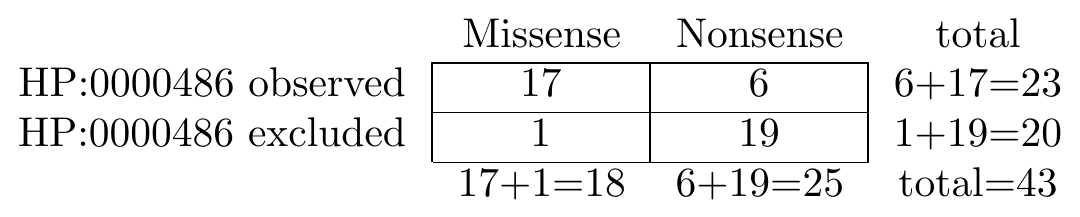
The following graphic shows an example contingency table that is used to conduct a Fisher exact test. We are comparing the frequency of strabismus in individuals with missense and nonsense variants:
To perform the corresponding test in Python, we would use the following code.
>>> import scipy.stats as stats
>>> contingency_table = [
... #   Missense,    Nonsense
...    [17,          6       ],  # Strabismus observed
...    [1,          19       ],  # Strabismus excluded
... ]
>>> oddsratio, p_value = stats.fisher_exact(contingency_table)
>>> float(oddsratio)
53.833333333333336
>>> float(p_value)
5.432292015291845e-06
The p_value evaluates to 5.432292015291845e-06, meaning there is a significant difference between the groups.
The Fisher exact test evaluates whether the observed frequencies in a contingency table significantly deviate from the frequencies we would expect if there were no association between the variables. We want to test whether the frequency of HP:0000486` is significantly higher or lower in one genotype group compared to what would be expected if there were no association. Note that by default, the two-tailed Fisher exact test is performed, meaning we have no hypothesis as to whether there is a higher or lower frequency in one of the genotype groups.
However, we are typically interested in testing the associations between the genotype and multiple phenotypic features at once. GPSEA takes advantage of the HPO structure and simplifies the testing for all HPO terms encoded in the cohort.
Example
Let’s illustrate this in a real-life example of the analysis of the association between frameshift variants in TBX5 gene and congenital heart defects in the dataset of 156 individuals with mutations in TBX5 whose signs and symptoms were encoded into HPO terms, stored as phenopackets of the GA4GH Phenopacket Schema, and deposited in Phenopacket Store (version 0.1.18).
Note
The shorter version of the same analysis has been presented in the Tutorial.
Create cohort
We will load and transform the phenopackets into a Cohort,
as described in Input data section. Briefly, we will load the phenopackets:
>>> from ppktstore.registry import configure_phenopacket_registry
>>> registry = configure_phenopacket_registry()
>>> with registry.open_phenopacket_store(release='0.1.18') as ps:
...     phenopackets = tuple(ps.iter_cohort_phenopackets('TBX5'))
>>> len(phenopackets)
156
followed by loading HPO release v2024-07-01:
>>> import hpotk
>>> store = hpotk.configure_ontology_store()
>>> hpo = store.load_minimal_hpo(release='v2024-07-01')
and we will perform Q/C and functional annotations for the mutations with the default cohort creator:
>>> from gpsea.preprocessing import configure_caching_cohort_creator, load_phenopackets
>>> cohort_creator = configure_caching_cohort_creator(hpo)
>>> cohort, qc_results = load_phenopackets(phenopackets, cohort_creator)
Individuals Processed: ...
>>> qc_results.summarize()
Validated under none policy
No errors or warnings were found
Configure analysis
We want to test the association between frameshift TBX5 variants and phenotypic abnormalities. GPSEA exposes a flexible predicate API that lets us create genotype and phenotype predicates to assign the cohort members into genotype and phenotype categories based on the variants and the HPO terms. We need to create one genotype predicate and one or more phenotype predicates.
Genotype predicate
We want to separate the patients into two groups: a group with a frameshift variant and a group without a frameshift variant, based on the functional annotation. We will use the MANE transcript for the analysis:
Building a genotype predicate is a two step process.
First, we create a VariantPredicate
to test if the variant leads to a frameshift (in this case):
>>> from gpsea.model import VariantEffect
>>> from gpsea.analysis.predicate.genotype import VariantPredicates
>>> tx_id = 'NM_181486.4'
>>> is_frameshift = VariantPredicates.variant_effect(VariantEffect.FRAMESHIFT_VARIANT, tx_id)
>>> is_frameshift.get_question()
'FRAMESHIFT_VARIANT on NM_181486.4'
and then we choose the expected mode of inheritance to test. In case of TBX5, we expect the autosomal dominant mode of inheritance:
>>> from gpsea.analysis.predicate.genotype import autosomal_dominant
>>> gt_predicate = autosomal_dominant(is_frameshift)
>>> gt_predicate.display_question()
'What is the genotype group: HOM_REF, HET'
gt_predicate will assign the patients with no frameshift variant allele into HOM_REF group and the patients with one frameshift allele will be assigned into HET group. Note, any patient with 2 or more alleles will be omitted from the analysis.
Note
Mode of inheritance testing is not the only way to dissect by a genotype. See the Genotype Predicates section for more info.
Phenotype predicates
We recommend testing the genotype phenotype association for all HPO terms that are present in 2 or more cohort members,
while taking advantage of the HPO graph structure and of the True path rule.
We will use the prepare_predicates_for_terms_of_interest()
utility function to generate phenotype predicates for all HPO terms:
>>> from gpsea.analysis.predicate.phenotype import prepare_predicates_for_terms_of_interest
>>> pheno_predicates = prepare_predicates_for_terms_of_interest(
...     cohort=cohort,
...     hpo=hpo,
...     min_n_of_patients_with_term=2,
... )
>>> len(pheno_predicates)
260
The function finds all HPO terms that annotate at least n (min_n_of_patients_with_term=2 above) individuals,
including the indirect annotations whose presence is implied by the true path rule.
Statistical test
We will use :ref:<fisher-exact-test> to test the association between genotype and phenotype groups, as described previously.
>>> from gpsea.analysis.pcats.stats import FisherExactTest
>>> count_statistic = FisherExactTest()
FET will compute a p value for each genotype phenotype group.
Multiple testing correction
In the case of this cohort, we could test association between having a frameshift variant and one of 260 HPO terms. However, testing multiple hypotheses on the same dataset increases the risk of finding a significant association by chance. GPSEA uses a two-pronged strategy to mitigate this risk - use Phenotype MTC filter and multiple testing correction.
Note
See the Multiple-testing correction section for more info on multiple testing procedures.
Here we will use a combination of the HPO MTC filter (HpoMtcFilter)
with Benjamini-Hochberg procedure (mtc_correction='fdr_bh')
with a false discovery control level set to 0.05 (mtc_alpha=0.05):
>>> from gpsea.analysis.mtc_filter import HpoMtcFilter
>>> mtc_filter = HpoMtcFilter.default_filter(hpo, term_frequency_threshold=0.2)
>>> mtc_correction = 'fdr_bh'
>>> mtc_alpha = 0.05
Final analysis
We finalize the analysis setup by putting all components together
into HpoTermAnalysis:
>>> from gpsea.analysis.pcats import HpoTermAnalysis
>>> analysis = HpoTermAnalysis(
...     count_statistic=count_statistic,
...     mtc_filter=mtc_filter,
...     mtc_correction=mtc_correction,
...     mtc_alpha=mtc_alpha,
... )
Analysis
We can now execute the analysis:
>>> result = analysis.compare_genotype_vs_phenotypes(
...     cohort=cohort,
...     gt_predicate=gt_predicate,
...     pheno_predicates=pheno_predicates,
... )
>>> len(result.phenotypes)
260
>>> result.total_tests
16
Thanks to Phenotype MTC filter, we only tested 16 out of 260 terms. We can learn more by showing the MTC filter report:
>>> from gpsea.view import MtcStatsViewer
>>> mtc_viewer = MtcStatsViewer()
>>> mtc_report = mtc_viewer.process(result)
>>> with open('docs/user-guide/report/tbx5_frameshift.mtc_report.html', 'w') as fh:
...     _ = fh.write(mtc_report)
Phenotype testing report
Phenotype MTC filter: HPO MTC filter
Multiple testing correction: fdr_bh
Performed statistical tests for 16 out of the total of 260 HPO terms.
| Code | Reason | Count |
|---|---|---|
| HMF01 | Skipping term with maximum frequency that was less than threshold 0.2 | 10 |
| HMF02 | Skipping term because no genotype has more than one observed HPO count | 4 |
| HMF03 | Skipping term because of a child term with the same individual counts | 1 |
| HMF04 | Skipping term because all genotypes have same HPO observed proportions | 50 |
| HMF05 | Skipping term because one genotype had zero observations | 5 |
| HMF06 | Skipping term with less than 7 observations (not powered for 2x2) | 130 |
| HMF08 | Skipping general term | 44 |
Genotype phenotype associations
Last, let’s explore the associations. The results include a table with all tested HPO terms ordered by the corrected p value (Benjamini-Hochberg FDR):
>>> from gpsea.view import summarize_hpo_analysis
>>> summary_df = summarize_hpo_analysis(hpo, result)
>>> summary_df.to_csv('docs/user-guide/report/tbx5_frameshift.csv')
What is the genotype group |
HOM_REF |
HOM_REF |
HET |
HET |
||
|---|---|---|---|---|---|---|
Count |
Percent |
Count |
Percent |
Corrected p values |
p values |
|
Ventricular septal defect [HP:0001629] |
42/71 |
59% |
19/19 |
100% |
0.003870827221893892 |
0.00024192670136836825 |
Abnormal atrioventricular conduction [HP:0005150] |
1/23 |
4% |
3/3 |
100% |
0.01230769230769231 |
0.0015384615384615387 |
Absent thumb [HP:0009777] |
18/100 |
18% |
14/31 |
45% |
0.01980624808543961 |
0.003713671516019927 |
Atrioventricular block [HP:0001678] |
1/23 |
4% |
2/2 |
100% |
0.04 |
0.01 |
Patent ductus arteriosus [HP:0001643] |
6/40 |
15% |
2/2 |
100% |
0.10406504065040649 |
0.03252032520325203 |
Secundum atrial septal defect [HP:0001684] |
23/55 |
42% |
4/22 |
18% |
0.15059037690969213 |
0.06544319142266644 |
Triphalangeal thumb [HP:0001199] |
23/99 |
23% |
13/32 |
41% |
0.15059037690969213 |
0.06932119159387057 |
Cardiac conduction abnormality [HP:0031546] |
15/37 |
41% |
3/3 |
100% |
0.15059037690969213 |
0.08259109311740892 |
Muscular ventricular septal defect [HP:0011623] |
8/84 |
10% |
6/25 |
24% |
0.15059037690969213 |
0.08470708701170182 |
Pulmonary arterial hypertension [HP:0002092] |
8/14 |
57% |
0/2 |
0% |
0.708378140298727 |
0.4666666666666667 |
Short thumb [HP:0009778] |
25/69 |
36% |
8/30 |
27% |
0.708378140298727 |
0.48700997145537483 |
Absent radius [HP:0003974] |
9/43 |
21% |
6/25 |
24% |
1.0 |
0.7703831604944444 |
Atrial septal defect [HP:0001631] |
63/65 |
97% |
20/20 |
100% |
1.0 |
1.0 |
Hypoplasia of the radius [HP:0002984] |
34/75 |
45% |
6/14 |
43% |
1.0 |
1.0 |
Hypoplasia of the ulna [HP:0003022] |
3/17 |
18% |
2/10 |
20% |
1.0 |
1.0 |
Short humerus [HP:0005792] |
8/21 |
38% |
4/9 |
44% |
1.0 |
1.0 |
The table shows that several HPO terms are significantly associated with presence of a heterozygous (HET) frameshift variant in TBX5. For example, Ventricular septal defect was observed in 31/60 (52%) patients with a missense variant but it was observed in 19/19 (100%) patients with a frameshift variant. Fisher exact test computed a p value of ~0.000242 and the p value corrected by Benjamini-Hochberg procedure is ~0.00387.
The table includes all HPO terms of the cohort, including the terms that were not selected for testing and thus have no associated p value.
Phenotype score
Mann-Whitney U Test
We may want to compare the total number of occurences of a specific set of phenotypic features between two different genotype groups. For instance, Jordan et al (2018) found that the total number of structural defects of the brain, eye, heart, and kidney and sensorineural hearing loss seen in individuals with point mutations in the Atrophin-1 domain of the RERE gene is significantly higher than expected based on the number of similar defects seen in individuals with putative loss-of-function variants. Since there are five potential defects, each individual has a count ranging between 0 and 5.
We perform a Mann-Whitney U Test (or Wilcoxon Rank-Sum Test) to compare the distribution of such counts between genotype groups. This is a non-parametric test that compares the medians of the two groups to determine if they come from the same distribution.
>>> import scipy.stats as stats
>>> group1 = [0, 0, 1, 0, 2, 0, 1, 1, 1, 0, 2, 0, 0, 3, 1, 1, 1, 0]
>>> group2 = [4, 5, 3, 4, 3, 3, 3, 4, 4, 5, 5, 2, 3, 0, 3, 5, 2, 3]
>>> r = stats.mannwhitneyu(x=group1, y=group2, alternative = 'two-sided')
>>> p_value = r.pvalue
>>> float(p_value)
6.348081479150902e-06
p_value evaluates to 6.348081479150901e-06, meaning there is a significant difference between the groups.
Example
Let’s now analyze the subjects reported in Jordan et al.
We will load 19 phenopackets that represent individuals with mutations in RERE
whose signs and symptoms were encoded into HPO terms and deposited into Phenopacket Store.
The phenopackets will be processed into Cohort
as described in the Input data section.
Briefly, we will first load 19 phenopackets
>>> from ppktstore.registry import configure_phenopacket_registry
>>> registry = configure_phenopacket_registry()
>>> with registry.open_phenopacket_store(release='0.1.18') as ps:
...     phenopackets = tuple(ps.iter_cohort_phenopackets('RERE'))
>>> len(phenopackets)
19
and load HPO (version v2024-07-01)
>>> import hpotk
>>> store = hpotk.configure_ontology_store()
>>> hpo = store.load_minimal_hpo(release='v2024-07-01')
to create a CohortCreator
>>> from gpsea.preprocessing import configure_caching_cohort_creator
>>> cohort_creator = configure_caching_cohort_creator(hpo)
which we will use to preprocess the cohort
>>> from gpsea.preprocessing import load_phenopackets
>>> cohort, _ = load_phenopackets(phenopackets, cohort_creator)
Individuals Processed: ...
resulting in a cohort consisting of 19 individuals
>>> len(cohort)
19
Configure analysis
Now we can set up the analysis of genotype and phenotype. We will perform the analysis using the RERE transcript selected as the “main” biologically relevant by the MANE consortium.
>>> tx_id = 'NM_001042681.2'
Genotype predicate
Jordan et al. compare phenotype of individuals harboring point mutations with the individuals carrying loss of function mutations. Let’s create a predicate for testing if the variant is a point mutation or a loss of function mutation.
In this example, the point mutation is a mutation that meets the following conditions:
predicted to lead to a missense variant on the MANE transcript
the Length of the reference allele is equal to 1
the Change length of an allele is equal to 0
>>> from gpsea.model import VariantEffect
>>> from gpsea.analysis.predicate.genotype import VariantPredicates
>>> point_mutation_effects = (
...     VariantEffect.MISSENSE_VARIANT,
... )
>>> point_mutation = VariantPredicates.change_length('==', 0) \
...     & VariantPredicates.ref_length('==', 1) \
...     & VariantPredicates.any(VariantPredicates.variant_effect(effect, tx_id) for effect in point_mutation_effects)
>>> point_mutation.get_question()
'((change length == 0 AND ref allele length == 1) AND MISSENSE_VARIANT on NM_001042681.2)'
For the loss of function predicate, the following variant effects are considered loss of function:
>>> lof_effects = (
...     VariantEffect.TRANSCRIPT_ABLATION,
...     VariantEffect.FRAMESHIFT_VARIANT,
...     VariantEffect.START_LOST,
...     VariantEffect.STOP_GAINED,
... )
>>> lof_mutation = VariantPredicates.any(VariantPredicates.variant_effect(eff, tx_id) for eff in lof_effects)
>>> lof_mutation.get_question()
'(TRANSCRIPT_ABLATION on NM_001042681.2 OR FRAMESHIFT_VARIANT on NM_001042681.2 OR START_LOST on NM_001042681.2 OR STOP_GAINED on NM_001042681.2)'
The genotype predicate will bin the patient into two groups: a point mutation group or the loss of function group:
>>> from gpsea.analysis.predicate.genotype import groups_predicate
>>> gt_predicate = groups_predicate(
...     predicates=(point_mutation, lof_mutation),
...     group_names=('Point', 'LoF'),
... )
>>> gt_predicate.display_question()
'Genotype group: Point, LoF'
Phenotype score
The authors score the individuals based on the number of structural defects from the following 5 categories:
Brain anomalies
Eye anomalies
Congenital heart defects
Renal anomalies
Sensorineural hearing loss
and they assign each individual a score based on the number structural defects. For example, an individual with a congenital heart defect would be assigned a score of 1, an individual with congenital heart defect and a renal anomaly would be assigned a score of 2, and so on.
We automatize this scoring method by encoding the categories into HPO terms
>>> structural_defects = (
...     'HP:0012443',  # Abnormal brain morphology (Brain anomalies)
...     'HP:0012372',  # Abnormal eye morphology (Eye anomalies)
...     'HP:0001627',  # Abnormal heart morphology (Congenital heart defects)
...     'HP:0012210',  # Abnormal renal morphology (Renal anomalies)
...     'HP:0000407',  # Sensorineural hearing impairment (Sensorineural hearing loss)
... )
and then test the individuals for presence of at least one HPO term that corresponds to the structural defect category (e.g. Abnormal brain morphology) or that is its descendant (e.g. Cerebellar atrophy).
GPSEA implements this scoring method in CountingPhenotypeScorer.
>>> from gpsea.analysis.pscore import CountingPhenotypeScorer
>>> pheno_scorer = CountingPhenotypeScorer.from_query_curies(
...     hpo=hpo,
...     query=structural_defects,
... )
Statistical test
We will use Mann-Whitney U Test as described above.
>>> from gpsea.analysis.pscore.stats import MannWhitneyStatistic
>>> score_statistic = MannWhitneyStatistic()
Tip
See gpsea.analysis.pscore.stats module for more statistical tests available
for using with phenotype scores.
Final analysis
We will put the final analysis together into PhenotypeScoreAnalysis.
>>> from gpsea.analysis.pscore import PhenotypeScoreAnalysis
>>> score_analysis = PhenotypeScoreAnalysis(
...     score_statistic=score_statistic,
... )
Analysis
We execute the analysis by running
>>> result = score_analysis.compare_genotype_vs_phenotype_score(
...     cohort=cohort,
...     gt_predicate=gt_predicate,
...     pheno_scorer=pheno_scorer,
... )
The analysis shows a significant difference between the number of structural defects in individuals with point vs. loss-of-function mutations.
>>> result.pval
0.012074957610483744
To explore further, we can access a data frame with genotype categories and phenotype counts:
>>> scores = result.genotype_phenotype_scores.sort_index()
>>> scores.head()
                                     genotype phenotype
patient_id
Subject 10[PMID_27087320_Subject_10]        1         0
Subject 1[PMID_27087320_Subject_1]          0         4
Subject 1[PMID_29330883_Subject_1]          1         0
Subject 2[PMID_27087320_Subject_2]       None         4
Subject 2[PMID_29330883_Subject_2]          1         1
The data frame provides a genotype category and a phenotype score for each patient. The genotype category should be interpreted in the context of the genotype predicate:
>>> gt_id_to_name = {c.category.cat_id: c.category.name for c in gt_predicate.get_categorizations()}
>>> gt_id_to_name
{0: 'Point', 1: 'LoF'}
The genotype code 0 is assigned to patients with a point mutation, 1 corresponds to the loss-of-function mutations, and None is assigned to patients who cannot be assigned into any of the groups.
Last, let’s use plot_boxplots() method
to show a box plot of the phenotype score distributions:
>>> import matplotlib.pyplot as plt
>>> fig, ax = plt.subplots(figsize=(6, 4), dpi=120)
>>> result.plot_boxplots(
...     gt_predicate=gt_predicate,
...     ax=ax,
... )
>>> _ = ax.grid(axis="y")
>>> _ = ax.set(
...     ylabel="Phenotype score", ylim=(-0.5, len(structural_defects) + 0.5)
... )
>>> fig.savefig('docs/img/rere_phenotype_score_boxplot.png')

We see that the individuals with the point mutations feature structural defects than the individuals with the loss-of-function mutations.
The box extends from the first quartile (Q1) to the third quartile (Q3) of the data, with a red line at the median. The whiskers extend from the box to the farthest data point lying within 1.5x the inter-quartile range (IQR) from the box.